20160228 Indiscrete mathematics

I’ve been fighting with the HTTPStime polling code, trying to minimize the number of requests we need to send to get a usable result.

The problem is a problem of discrete mathematics with hard boundaries, and I’m not good at that.

The ideal case is that we send the first request right after the second changed on the server, and we receive the second response right before the second changes on the server.

That is only possible if we already know what we are trying to measure, and if we happen to send the first request a tad too early or the second request a tad too late, we get worst case results instead.

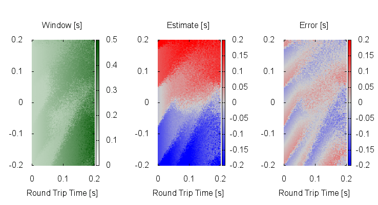
Trying to be smart about it, one easily ends up with functions which if built as roof over a museum would win an architectural prize. Here is one such example:

The leftmost plot shows how big our final window is for a given RTT and clock offset.

The middle plot shows our estimate of the time difference using the middle of the window and that’s almost even worse.

The rightmost plot shows the error, and it is readily obvious that there are significant biases around the most important “No clock skew, nearby server” space.

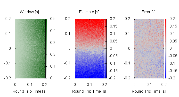
Here on the other hand, is a four-volley result for the totally naïve algorithm of “aim for the middle with a little twist”:

Much better. Not flat, but no systematic biases either.

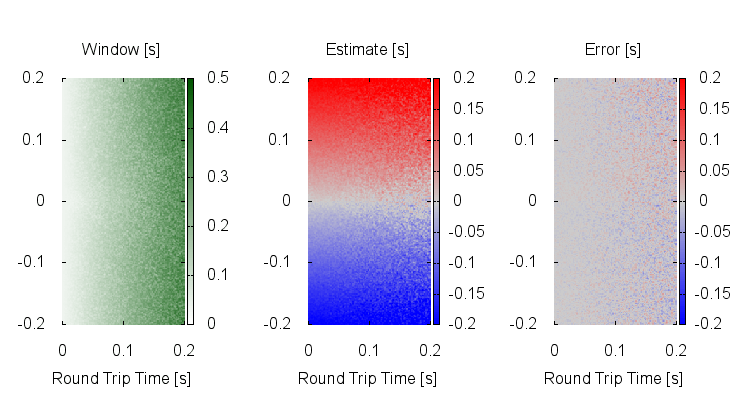
If we allow two more volleys, for a total of six, the result improves noticeably:

The little twist is that once we know the RTT - after the second volley since the first one has the TLS/SSL negotiation overhead - we pick which end of the volley to probe with, depending on the sign of the aimpoint.

To be perfectly honest: I have no idea why that works better than using either end of the volley every other time, but it is about 10% better.

I’ll be very interested if anybody can improve this result.

…or even just explain it.

phk

Here is the python code which simulates the HTTPstime protocol:

#!/usr/bin/env python

from __future__ import print_function

import random

def shot(t1, rtt, off):
        ltx = t1
        rrx = ltx + .5 * rtt
        ts = rrx - off

        # Jitter (RTT + measurement)
        ts += random.uniform(-5e-3, 5e-3)

        ts = int(ts)
        rtx = rrx
        lrx = rtx + .5 * rtt
        return (ltx, ts, lrx, ltx - ts - 1, lrx - ts)


xres = 150
yres = 300

fo = open("/tmp/_", "w")
for i in range(xres):
        rtt = i * .2 / (xres-1)

        for j in range(yres):
                off = -.2 + j * .4 / (yres-1)

                # RTT on first packet is larger
                # And we have no idea when it gets sent
                x = shot(random.uniform(1,2), rtt * random.triangular(1,3), off)
                l = x[3]
                h = x[4]

                for i in range (3):     # Npacket - 1

                        # Aim for the middle
                        m = (h + l) * .5

                        if i > 0 and m > 0:
                                m -= (x[2] - x[0])

                        x = shot(2.00 + m, rtt, off)
                        l = max(l, x[3])
                        h = min(h, x[4])

                z = h - l
                m = (h + l) * .5

                fo.write("%.3f %.3f %.3f %.3f %.3f\n" % (rtt, off, z, m, m-off))
        fo.write("\n")

And here is the gnuplot script to plot the result:

set size ratio -1
set xtics .1
set ytics .1
set border 0

set pm3d map
set xlabel "Round Trip Time [s]"
set ylabel "Clock Offset [s]"

set title "Window [s]"
set cbrange [0:.5]
set palette defined  (0 "#ffffff", 1 "#005500")

set term wxt 0
splot '/tmp/_' using 1:2:3 notitle

set term png size 240,400
set output "/tmp/_1.png"
replot
set output

set title "Estimate [s]"
set palette defined (-1 "#0000ff", 0 "#cccccc", 1 "#ff0000")
set cbrange [-.2:.2]

set term wxt 1
splot '/tmp/_' using 1:2:4 notitle

set term png size 240,400
set output "/tmp/_2.png"
replot
set output

set title "Error [s]"
set term wxt 2
splot '/tmp/_' using 1:2:5 notitle

set term png size 240,400
set output "/tmp/_3.png"
replot
set output

!montage /tmp/_[123].png -geometry +3+1 /tmp/x.png

!ministat -n -C5 /tmp/_